Site and fleet
Compute–electricity coordination makes wind, solar and battery supply with limited biomethane backup cheaper than grid electricity in the Lanarkshire study. Under a 10% biomethane budget, the selected design costs £2.41M per year With coordination, compared with £6.50M Without coordination and a £2.81M grid bill at the default prices. At a 15% budget, coordination likewise lowers the selected design's cost from above to below the grid bill.
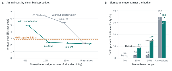
Figure 1. Coordination brings the limited-biomethane designs below the default grid bill. a, Annual cost of the selected design at each biomethane budget, Without coordination and With coordination. Short bars mark the mean of the three design years 2020, 2022 and 2023; dots show the individual years. Wind, solar and battery supply alone (0%) was selected With coordination only. The dashed line is the £2.81M grid bill at 19.1 p/kWh with the AI Growth Zone discount switched off. b, Share of site electricity supplied by biomethane engines. Dotted lines mark the 10% and 15% budgets, which limit the mean share across the design years. Costs use 4.98 p/kWh gas and the original battery costs, and include equipment, backup energy, lost service and the closing position of each run.
FilesSVGPDFPNG · 600 dpi
The study represents a hypothetical new data centre near the Lanarkshire AI Growth Zone in Scotland, with 3 MW of design IT capacity. The fleet comprises 1,648 B300 GPUs in 206 nodes and 1,152 RTX PRO 6000 Blackwell Server Edition GPUs in 144 nodes, with eight cards per node. The design capacity covers the servers and shared IT infrastructure. Actual demand follows the work running on the fleet and the overhead of keeping that equipment available.
The two GPU tiers retain their different physical characteristics. B300 is represented in an HGX system with HBM memory, NVSwitch within each node and a high-bandwidth network between nodes. RTX PRO 6000 uses GDDR7 memory and PCIe server infrastructure. Separate power and workload mappings for these tiers allow the same quantity of requested GPU time to produce different execution times, occupied capacity and energy use. Both tiers contain a mixture of task classes.
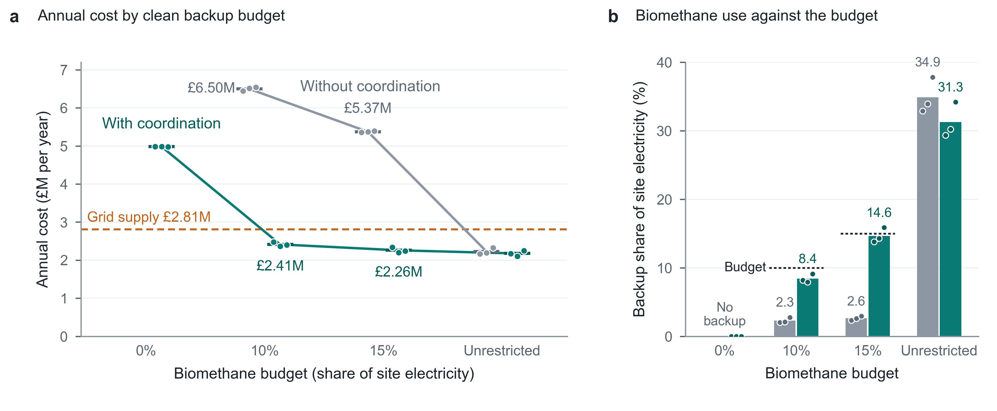
The model follows the connection between computing service and the equipment needed to supply it. Task arrivals and completions determine GPU and server demand; cooling, power distribution and auxiliaries complete the site load. Wind, Solar PV, Battery power, Battery energy and Backup engines then define the available supply. The Annual digital twin compares the resulting equipment costs and annual operation, while the weekly simulation exposes task placement, power and service outcomes within a chosen design.
Figure 2. Computing requirements and physical supply meet in hourly site operation. Card and node power translate the task workload into IT demand; cooling, distribution losses and auxiliaries complete the site boundary. Coordination uses arrived tasks, completion windows, a seven-day wind and solar forecast and the current work, node and battery state. Realised wind and solar output determine the supply available during operation. Solid arrows are model relationships; dashed arrows are operating controls over task timing, powered nodes, card power and battery charging. Equipment costs, fuel use and service outcomes together form the annual comparison.
FilesSVGPDFPNG · 600 dpi
Grid supply establishes the purchase-price comparison for the same reference site. The default case treats the data centre as a large customer within a Lanarkshire campus, using £108/MWh wholesale electricity with the AI Growth Zone discount switched off. This gives approximately 19.1 p/kWh and £2.81M per year at about 14.7 GWh annual reference demand. The comparison therefore asks whether coordinated renewable supply can beat a specified electricity bill while keeping biomethane use within the chosen budget.
Task sources
The scope for coordination begins with the services that the computing workload must deliver. Alibaba GPU cluster records preserve variation in task arrivals, durations, GPU requests and task classes. Mapping this demand to the UK fleet produces approximately 18 million tasks over a model year. Training, Offline inference, Online inference, Development, Other and Unlabelled remain distinguishable, so the supply comparison retains the difference between work that can wait and services that require immediate capacity.
Hardware conversion reflects the way each class delivers its service. For finite computations such as Training and Offline inference, the requested parallel GPU count is retained and execution time changes with the destination hardware. Online inference keeps its service period while its GPU allocation is resized to meet both computational demand and service memory requirements. Development keeps its reservation duration and uses a supported GPU partition on the destination tier. An upgrade can therefore shorten a computation or reduce a continuing service's device allocation, depending on the work involved.
The mapping uses benchmark-informed throughput relationships for the source and destination cards, with separate evidence for task and model types. Online services occupy discrete supported GPU partitions, including whole cards where required. Their allocation accounts for model and service memory as well as activity, so a low average computation rate can still require substantial device capacity. Demand from anonymised source accelerators uses an explicitly assumed hardware proxy.
Time flexibility is attached to the study's service requirements. Training and Offline inference can wait within a Completion window; Online inference and the remaining classes use Run at release. Continuing services therefore retain their required operating periods, while eligible finite computations can move within their completion allowances. The value of coordination depends on the mix of tasks and the time available to finish them.
Power at each card
GPU power distinguishes allocated capacity from active computation. A board can be in deep idle, hold a resident task context while computation is inactive, or execute active work. Task class, occupied share, source activity and card type determine the incremental draw above the board's idle requirement. Fractional tasks share a physical card, whose standing consumption is counted once. A task can therefore occupy memory and capacity while drawing less power than another task with the same GPU allocation.
The active-power response connects workload flexibility to electricity demand. Source task activity is used where available, with estimates by class and card for other tasks. Workload power relationships are anchored in H100 measurements and checked against published Blackwell measurements; online-service activity also varies within the day. These distinctions determine how much demand moves when a particular task is delayed, accelerated or capped.
Node power includes the server needed to support eight accelerators. Host processors and memory, local storage, interconnects, network interfaces, fans and power-supply losses contribute alongside the GPU boards. Shared networking, storage and management equipment then form the IT-room total. Host and infrastructure demand follow the model's hardware and allocation assumptions. Consolidating work onto fewer powered nodes can consequently save server overhead as well as GPU idle energy.
Site energy
The facility model follows the heat produced by each hardware tier. In the main configuration, direct liquid cooling serves the B300 nodes with 40°C facility-water supply, while 24°C supply air serves the remaining heat. Most B300 node heat enters the liquid loop; residual B300 heat, RTX nodes and shared IT equipment enter the air side. Coolant distribution units, pumps and dry coolers provide liquid-side heat rejection, with mechanical cooling when outdoor conditions require it. The air side accounts for chilled-water cooling, fans and pumps.
A shift in computing demand also changes the electricity needed to remove its heat. Hourly outdoor weather and the heat load determine the effort required to maintain the chosen supply-water and supply-air temperatures. The model also represents the effect of those temperature settings on server fans and board power. The site load therefore follows both the scheduled IT work and the facility's response to that work.
Power distribution and auxiliary services complete the site boundary. Transformer, UPS, cabling and distribution-unit losses are represented separately, together with lighting, building controls, security, office loads and standby-generator heating. Indoor distribution losses contribute to the air-side heat load. The reference facility account contains approximately 13.53 GWh of IT electricity, 0.31 GWh of cooling, 0.63 GWh of distribution losses and 0.25 GWh of auxiliaries per year, with rounding in these component totals.
PUE
PUE describes the facility overhead accompanying the computing workload. The main configuration gives approximately 14.7 GWh annual site electricity and a PUE of 1.088 for the reference workload with nodes kept on, averaged over ten weather years. PUE expresses total facility electricity relative to IT electricity. GPU execution, resident tasks and idle server overhead remain inside the IT account. Task-level power and node operation identify the demand available for coordination within that account.
Coordination levers
Coordination changes the timing of demand, the hardware kept on and the power used to make progress. These three controls let the fleet respond to renewable availability within the service requirements of its tasks. Their economic effect appears in the combination of supply equipment, backup use and delivered computation.
Deferral moves eligible computation within its Completion window. The window is measured from the finish time a task would have under Run at release. A task requiring four hours at full speed with a 24-hour window can finish up to 24 hours after that original finish time. The default allowances are 168 hours for Training and 24 hours for Offline inference, with class-specific alternatives available in the interface. This gives the scheduler a defined amount of time in which to align work with supply.
Node power states reduce the overhead of keeping spare hardware on. Work within each GPU tier can be consolidated onto the nodes that remain powered, allowing empty nodes to switch off while capacity is retained for running work and reserve. The operating rules normally require at least two hours on, one hour off and at most two starts in a rolling 24 hours. Task and reserve requirements can bring nodes on earlier. These conditions give switching a duration and a capacity consequence, as well as an energy saving.
Power capping trades lower task power against slower progress. The interactive simulation uses a 70% card-power setting for flexible work when the plan selects it. Its effect on progress depends on the card and workload, so the energy consequence reflects both the power reduction and the time required to complete the computation. Completion windows and available GPU capacity determine how much of this trade-off the site can use.
The three switches make their operating effects separately examinable. Deferral changes when work runs, Node power states changes how much hardware stays available, and Power capping changes the power and progress of running work. Paired weekly runs hold tasks, weather and supply equipment fixed. Backup generation, completed work and the end-of-week position then show what each selected combination achieves.
Scheduler decisions
Coordination operates with a finite view of future renewable supply. Each hourly plan uses a seven-day wind and solar forecast, tasks that have arrived, their remaining work and completion windows, available nodes and the battery state. It sets the amount of flexible work to run, the number of nodes on, the use of power capping and a battery target. Subsequent hours update those decisions as tasks progress and the supply outlook changes. The annual costs thus include the consequences of operating with the forecast available at each decision.
The plan balances electricity use with the consequences for service. Renewable-rich periods can accommodate more eligible work and battery charging; a poor supply outlook can favour waiting, lower task power or conservation of stored energy. Nearer completion limits reduce the scope to wait. Backup-energy prices and the Value of a GPU-hour affect the relative cost of consuming fuel and losing service, while the operating requirements of immediate tasks retain priority.
Realised supply determines how the plan is delivered. Wind and solar output, battery power and stored energy, and backup capacity together support the site's demand. When available supply falls short, eligible flexible work can be paused before a remaining electricity shortage is recorded. Interrupted work, task progress and battery state carry into later decisions. The resulting hourly record shows how forecast-based plans perform under the actual weather sequence used in the scenario.
Annual digital twin
The Annual digital twin tests whether a supply design can turn workload flexibility into a lower annual cost. The interface presents the design years 2020, 2022 and 2023, each with 8,760 hourly operating steps and the full site's task workload. Wind and solar capacity, battery power and energy, and backup-engine capacity determine the resources available in each hour. Task execution and facility demand determine how those resources are used.
The annual comparison includes equipment selection as well as operating decisions. Without coordination uses Run at release with nodes kept on; With coordination enables the task and node controls in the annual study. The supply design search selects equipment for each case. The nine displayed scenarios cover Natural gas, unrestricted Biomethane, Biomethane budgets of 10% and 15%, and wind, solar and battery supply alone. The limited-biomethane pairs establish the main economic comparison; the other cases show how it changes when more backup is permitted or backup is removed.
The current annual results use the selected equipment in fresh operating runs at the updated fuel prices. The same designs are also run through 2024 and 2025 as reporting years and 2021 as a held-out year. This extends the assessment from the years used to select equipment to three further weather sequences. The interface's heatmaps retain the three design years; the additional annual results establish how costs and fuel dependence change beyond them.
Annual cost combines the equipment commitment with its operating consequences. Wind, solar, battery and backup capacity contribute annualised costs; backup energy and lost service depend on the realised run. A closing settlement accounts for remaining work and the battery's ending position. Displayed summary values average the three design years, while the individual years retain their energy, service and hourly records. The displayed p/kWh uses the fixed reference annual site demand, keeping a common denominator across designs. Reading those quantities together distinguishes inexpensive supply from supply that also delivers the required service.
Annual service records show the computation delivered alongside the supply cost. All 27 displayed design-year runs record zero Unserved energy. Failed work remains a separate measure of tasks lost through capacity, timing or interruption. The cost breakdown includes a value for lost service and a closing settlement for unfinished work and battery depletion. The comparison therefore accounts for obligations left at the end of the run as well as electricity consumed during it.
The emissions account follows the fuel used in operation. Backup generation is valued with the selected fuel's emissions factor, and the grid comparison uses the matching weather year's national hourly carbon intensity. The current gas factor represents direct combustion emissions; the biomethane factor primarily represents upstream fuel supply under the study's renewable-gas certificate accounting. These fuel-specific boundaries define the carbon quantities alongside the economic and operational comparison.
Cost against the clean backup budget
Limited biomethane backup is the setting in which coordination changes the economic choice between renewable supply and the grid. At the default prices, the selected 10% and 15% designs Without coordination cost roughly 2.3 and 1.9 times the grid bill. With coordination, both fall below it. These comparisons combine the equipment selected for each case with its hourly operation and service costs.
| Biomethane budget | Without coordination | With coordination | With coordination relative to Grid supply |
|---|---|---|---|
| 10% | £6.50M/year | £2.41M/year | 14% lower |
| 15% | £5.37M/year | £2.26M/year | 20% lower |
These values average the three design years at 4.98 p/kWh gas, the original battery costs and a £2.81M annual grid comparison. The clean backup budget limits the mean share of site electricity supplied by biomethane engines across those years. It sets the permitted fuel dependence, while engine capacity remains a separate design choice. A small annual fuel allowance can still require substantial engine power during a short period of low renewable output.
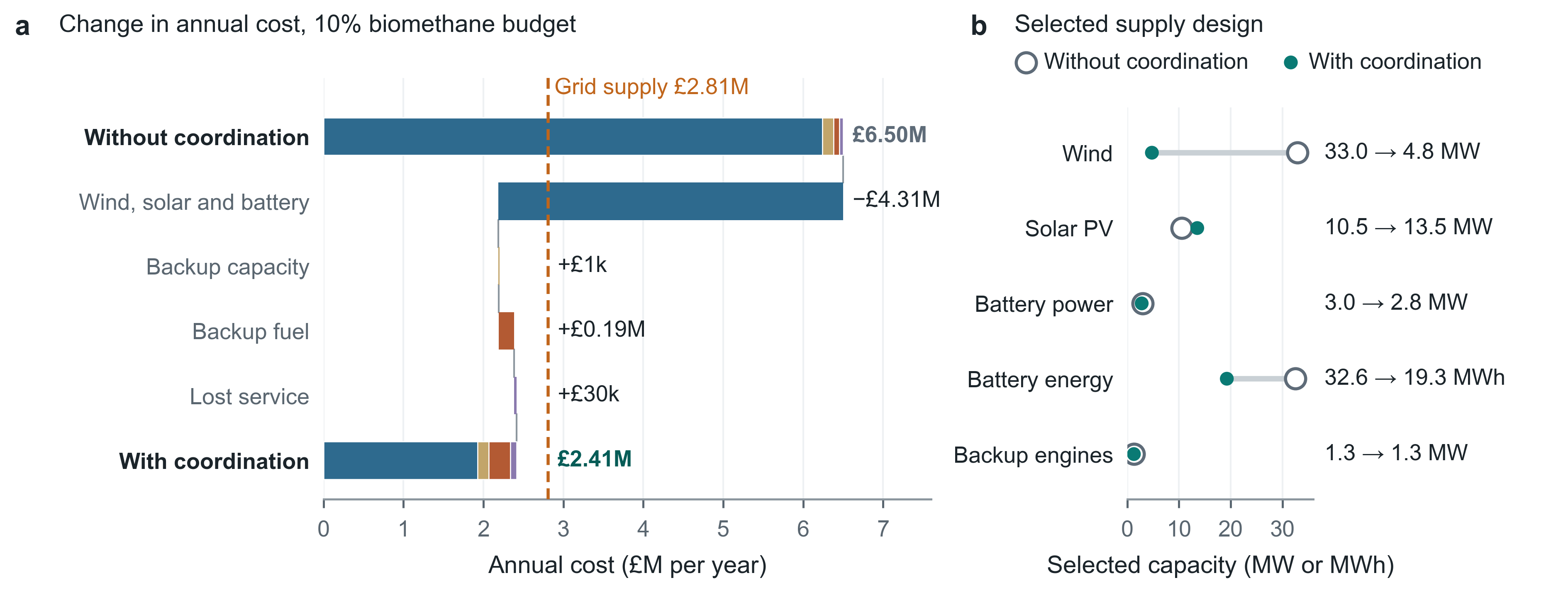
The equipment account explains most of the cost difference. In the 10% cases, annualised wind, solar and battery costs fall from approximately £6.24M Without coordination to £1.93M With coordination. The selected wind capacity falls from about 33.0 MW to 4.8 MW and battery storage from 32.6 MWh to 19.3 MWh, while solar capacity rises from 10.5 MW to 13.5 MW. Coordination is associated with a different supply mix and a much smaller annual equipment commitment. The remaining cost items record backup capacity, fuel use, lost service and the closing position of the run.
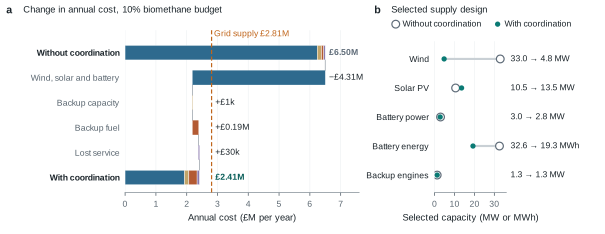
Figure 3. The smaller equipment commitment accounts for most of the cost difference in the 10% cases. a, Mean annual cost Without coordination (top bar) and With coordination (bottom bar), divided into Wind, solar and battery, Backup capacity, Backup fuel including the closing settlement, and Lost service; the rows between show the change in each component. Annualised wind, solar and battery costs fall by £4.31M, from £6.24M to £1.93M, while backup fuel rises by £0.19M. b, Capacities of the two selected designs. Values average the design years 2020, 2022 and 2023 at the default prices; the comparison includes both the selected supply equipment and its operation.
FilesSVGPDFPNG · 600 dpi
The lower equipment cost accompanies greater use of the available biomethane allowance. In the 10% designs, backup supplies a mean 2.3% of site electricity Without coordination and 8.4% With coordination. Mean Failed work is approximately 7,500 and 29,100 GPU-hours per year respectively, with its cost included in the annual account. The main saving therefore comes from the equipment commitment, alongside differences in fuel use and task service.
The cost plot connects these economic results to the operating evidence. Each point represents a selected design at its chosen backup budget; separate lines join the Without coordination and With coordination cases. Selecting a point opens the equipment, cost breakdown, achieved backup share, service outcomes and hourly record. The controls expose both sides of the result: the large equipment commitment in the uncoordinated designs and the operating performance of the less costly coordinated designs.
An unrestricted biomethane supply gives a different economic comparison. Its design Without coordination already costs about £2.23M per year, below the default grid bill, while using backup for roughly a third of site electricity. The 10% and 15% cases place a tighter condition on fuel dependence. Their much larger cost difference shows why the value of coordination is particularly consequential when backup energy is limited.
Complete removal of backup raises the equipment commitment again. The selected wind, solar and battery-only design With coordination contains approximately 97 MWh of battery storage and costs £4.98M per year in the design years, about 77% above the default grid bill. The lower-cost limited-biomethane designs occupy the middle ground between substantial fuel dependence and renewable supply with storage alone.
The selected 10% design retains its cost advantage in the additional weather years. Mean annual cost in 2024 and 2025 is £2.55M With coordination and £6.73M Without coordination; in 2021 the corresponding costs are £2.54M and £6.71M. The coordinated design uses biomethane for 9.8% of site electricity on average in 2024 and 2025 and 11.0% in 2021. It also records about 7 kWh per year of mean Unserved energy in 2024 and 2025. These runs expose the year-to-year fuel and supply requirements accompanying the cost result, including a year above the budget used to select the design.
Prices
The price controls identify the conditions under which coordinated supply remains cheaper than the grid. Gas price and Battery cost revalue each design and its saved operation, updating the cost plot, scenario cards and annual breakdown. Equipment, electricity quantities and task outcomes stay attached to those runs. A change in the cost ranking therefore describes price exposure for the displayed designs; the controls retain their selected equipment and schedules.
Gas price is expressed per unit of gas on a gross calorific value basis. The model translates it into a cost per unit of engine electricity using the engine's fuel requirement and the study's per-unit charges. Biomethane includes an assumed renewable-gas certificate premium. At the default gas price of 4.98 p/kWh, the resulting backup-energy prices are approximately £153.8/MWh for Natural gas and £219.8/MWh for Biomethane. Gas price and Wholesale electricity price can be varied independently.
Grid price combines wholesale electricity, a purchasing markup, policy and network charges, other stated adders and the selected AI Growth Zone discount. The default 19.1 p/kWh case assumes £108/MWh wholesale electricity with the discount switched off. Listed cases span approximately 11.8–19.1 p/kWh. They provide defined purchase-price conditions against which the off-grid system is compared.
A lower grid purchase price narrows the economic advantage. Across all six weather years, the selected 10% design With coordination costs about £2.48M per year, approximately 12% below the default grid bill. The alternative grid cases give about £2.46M with the AI Growth Zone discount at £108/MWh wholesale electricity, and £2.39M at £80/MWh without the discount. Those cases place the coordinated design close to or above the grid bill. The interface applies these grid-price choices to its comparison over the three design years.
Prices in Scheduling simulation enter a new operating calculation. Backup fuel prices the electricity supplied by the engine, and Value of a GPU-hour values service separately for B300 and RTX PRO 6000 work. Both are held constant within the selected week. Run the week applies the revised prices to planning and cost accounting, so the resulting task schedule and supply use can change as well as the bill.
Hourly operation
Hourly operation reveals how a design sustains supply through the conditions behind its annual cost. Each heatmap cell represents one hour, with days across the horizontal axis and hours of the day down the vertical axis. Selecting a weather year retains the sequence of renewable conditions, battery use and site demand that produced that year's result.
Backup generation and Battery energy show how supply is sustained through renewable shortfalls. Site load shows when the facility requires electricity, while Curtailed shows available renewable energy left unused. With coordination also provides B300 nodes on. Together these views can distinguish a recurring daily pattern from a prolonged low-renewable period and show whether flexible computing, stored energy or backup generation carries the response.
Scheduling simulation
Scheduling simulation examines the operational contribution of coordination within a fixed supply design. It uses the annual model's scheduling rules on one module over one week, with tasks taken from the site's selected nodes and the corresponding facility power characteristics. The browser evaluates the same tasks, weather and supply twice. Without coordination uses Run at release with nodes kept on; With coordination activates the selected Coordination levers. This comparison isolates changes in operation, while the annual study also compares the equipment selected for each case.
Weather week provides four contrasting supply conditions: Typical autumn week, Calm sunny week, Calm winter week and Windy winter week. Each selection includes the corresponding week's tasks and weather. Its paired runs isolate the effect of coordination for those inputs; comparison across weeks shows how the controls perform under different combinations of task demand and renewable supply.
Supply (site level) defines the equipment for the whole site, and the module receives its energy-based share. Battery power determines the rate at which storage can support a shortfall; Battery energy determines the amount available over time. Backup engines adds a further capacity limit, with Natural gas, Biomethane, Bio-LNG, HVO or Hydrogen as fuel choices. The default supply uses the Biomethane ≤ 10% design With coordination. A completed annual design can be transferred through Run this design in the scheduling simulation for examination under a selected week; a transferred design takes the place of that default.
Run the week calculates a new comparison after the settings change. The page first runs the default module automatically, then retains the completed result until another run is requested. The displayed results therefore correspond to the settings used for that calculation, including the weather, tasks, supply, levers and prices.
Module and task volume
Module and task volume determine how much eligible work is available to respond to supply. The default module contains four B300 nodes and four RTX PRO 6000 nodes, totalling 64 GPUs and approximately 2.1% of reference site electricity. Each tier can use one to eight nodes. Tasks come from the full-site schedule's selected nodes, preserving their timing, GPU requests and class mix within the module.
Task volume changes the demand placed on that module by class. Training, Offline inference and Online inference have separate multipliers, while Development, Other and Unlabelled share a fourth control. The range is zero to twice the original volume. Above the original volume, additional tasks enter where they fit under full-speed operation; the interface also reports extra tasks without room. This separates the demand admitted to the comparison from the requested increase in work.
Week results and week cost
Week results places electricity savings alongside completed computing service. Difference consistently means With coordination minus Without coordination. Site energy and Backup generation describe the electricity effect; Completed work, Work carried into next week, Failed tasks and Interruptions describe delivery and disruption. These measures identify whether a lower weekly cost accompanies changes in completed outputs, service failures or work left to finish.
| Measure | Interpretation |
|---|---|
| Site energy | Modelled electricity demand of the module at the site boundary |
| Wind and solar available | Renewable generation available to the module before curtailment |
| Backup generation | Electricity supplied by backup engines |
| Curtailed | Available renewable energy used by neither the load nor battery charging |
| Battery discharge | Energy delivered from storage to the load |
| Unserved energy | Remaining electricity shortfall after eligible flexible work has been paused |
| Completed work | Full requested GPU-hours of tasks recorded as completed |
| Work carried into next week | Remaining work of released tasks still active or waiting at the week's end |
| Failed tasks | Number of tasks recorded as failed during the week |
| Interruptions | Number of interruptions to task execution |
| Mean nodes on | Time-average count of powered nodes for each GPU tier |
Completed work accounts for task outputs. A task already active at the start of the week contributes its full requested work if it finishes during the week, while carry-over records the remaining work of tasks still awaiting completion. These quantities connect the electricity consumed during the comparison to completed outputs and outstanding work.
Failed tasks and Interruptions identify disruption to service. Tasks can fail when required GPU capacity is unavailable at their latest feasible start, or when an interruption leaves too little time for recovery and completion. Electricity shortages affecting protected immediate work appear separately as Unserved energy. Task outcomes and supply adequacy are therefore assessed together.
Week cost places supply investment and operating consequences on a common weekly basis. Wind, solar and battery and Backup capacity are the module's share of annual equipment costs allocated to the simulated period. Backup fuel follows simulated engine generation. Lost service values failed task work and the service associated with unmet electricity demand using the selected GPU-hour values. The total covers these supply and service items; GPU purchases, staffing and commercial revenue belong to a broader data-centre business account.
End-of-week settlement accounts for obligations left at the comparison boundary. It prices the estimated energy required by remaining work, together with battery energy below the initial level, at the selected backup-energy price. A battery ending above its initial level attracts zero depletion charge. This closing adjustment puts deferred work and battery depletion into the same weekly cost comparison while their physical state remains visible in the service and storage results.
Card view
Card view exposes the task placements through which the demand profile changes. Each row represents one GPU, with task bars arranged within its node along the time axis. Switching between Without coordination and With coordination connects aggregate power to the timing of individual tasks, occupied capacity and the number of nodes kept on. Deferral, consolidation and capped execution can be examined on the hardware that carries the work.
Colour identifies task class: green for Training, blue for Offline inference, orange for Online inference, purple for Development, brown for Other and grey-green for Unlabelled. Lighter task bars indicate Capped operation, and grey bands indicate Node off. A long task bar in a lower-power state can therefore be distinguished from an empty period or a node that has been switched off.
The task readout connects visible placement to its service record. Hovering over a bar exposes the task class, GPU request, card type, Release, Start and Status, together with the applicable End, Deadline and interruption information. The Power and Battery energy charts place that same operating period in its electricity context.
Task table
Task table extends the weekly comparison to a specified workload. A supplied CSV replaces the module's original tasks, with one row per task on the chosen fleet. Uploaded tasks use a common average power per requested GPU within each tier; flexible tasks also use that tier's average power and progress changes under capping. The original trace-derived task set retains its richer activity information. Changes in task mix and timing can then be assessed through the same paired energy, cost and service results.
| Column | Content |
|---|---|
release_h | Release time in hours relative to the start of the week; a negative value represents a task already running with prior full-speed progress |
duration_h | Positive duration in hours at full speed |
gpus | Requested GPU quantity or fraction greater than zero and up to eight |
card | B300 or RTX |
class | training, offline_inference, online_inference, dev, other or unknown |
The upload reads up to 20,000 data rows in a simple comma-separated format. The loaded count reports parsed records; eligibility for the weekly run also depends on GPU quantity and release before hour 168. Uploaded rows determine Task volume directly. Use the site's tasks restores the original workload and its volume controls.
Full-year run
Full-year run evaluates whether coordinated renewable supply with a limited backup allowance is economical for a specified site. The complete model runs on a workstation, combining location and weather years, GPU and node hardware, shared IT and facility loads, task records and service requirements, and the available generation, storage and backup options. Supply costs and grid-price assumptions establish the comparison for that site.
The annual analysis identifies supply designs that meet the site's chosen economic and operating criteria. It assesses equipment costs, fuel dependence and service outcomes across weather years; the browser's weekly comparisons, hourly views and card records expose how selected operation uses resources and delivers work. Applying this assessment to another site makes the same economic question specific to its workload, hardware, weather, prices and acceptable service outcomes. Enquiries for a site-specific annual calculation can be sent to hx279@cam.ac.uk.